
This post is the fourth and final post in this series. Here we will query the database in a couple of different ways and perform some visualisation of the data.
SQL Queries using MySQL
After creating and loading the data into the database, we can now query it. Queries can be posed by typing the SQL commands directly into the MySQL terminal or
by writing them in a file, which would then be run from the terminal using the
SOURCE command. In the file SQL_Queries_1.sql we consider many questions and answer them
by querying the IMDb database. This section is an on going piece of work and we
intend to add more queries to the repository in the future.
For each query in the file SQL_Queries_1.sql we create a view by
CREATE OR REPLACE VIEW Q1(column_1,column_2)
AS
...
;
The result of the query which is stored in the view can be seen by
SELECT * FROM Q1;
To delete the view
DROP VIEW Q1;
The database is quite large, so for illustration purposes we will quite often limit ourselves to the first few entries only.
A few example queries
We will consider a few queries for illustration purposes.
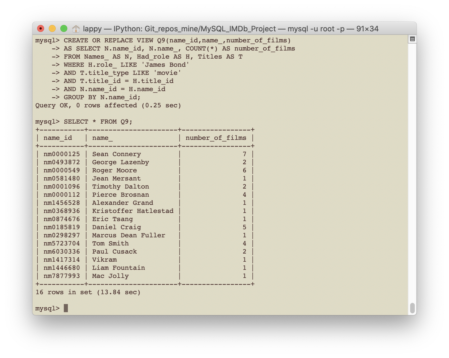
- Query 9: Who are the actors who played James Bond in a movie? How many times did they play the role of James Bond?
CREATE OR REPLACE VIEW Q9(name_id,name_,number_of_films)
AS SELECT N.name_id, N.name_, COUNT(*) AS number_of_films
FROM Names_ AS N, Had_role AS H, Titles AS T
WHERE H.role_ LIKE 'James Bond'
AND T.title_type LIKE 'movie'
AND T.title_id = H.title_id
AND N.name_id = H.name_id
GROUP BY N.name_id;
To see the results of this query:
SELECT * FROM Q9;
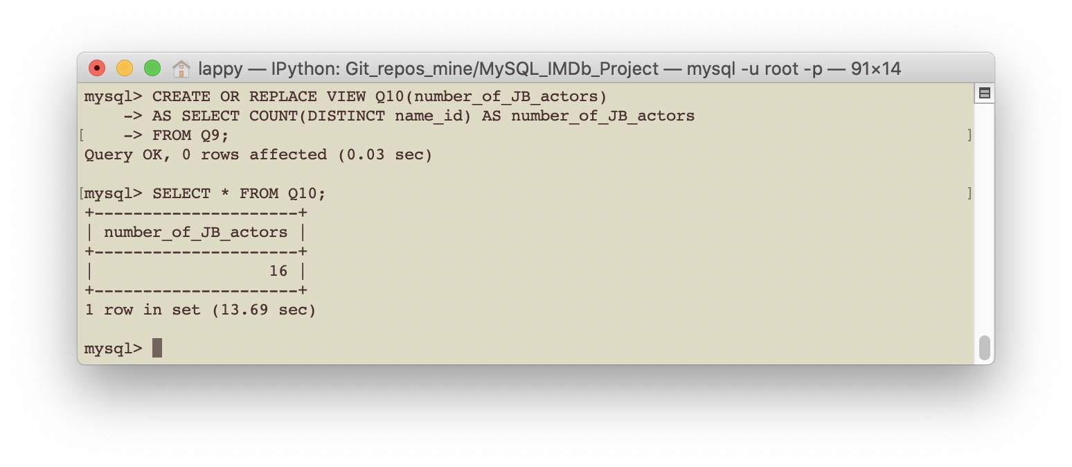
- Query 10: How many actors played James Bond?
CREATE OR REPLACE VIEW Q10(number_of_JB_actors)
AS SELECT COUNT(DISTINCT name_id) AS number_of_JB_actors
FROM Q9;
To see the results of this query:
SELECT * FROM Q10;
- Query 11: I don’t recognise some of the names shown above, so lets look at them more closely!
CREATE OR REPLACE VIEW Q11(name_,title_id,primary_title,start_year)
AS SELECT Q9.name_, T.title_id, T.primary_title, T.start_year
FROM Q9, Titles AS T, Had_role AS H
WHERE Q9.name_id = H.name_id
AND H.role_ LIKE 'James Bond'
AND T.title_id = H.title_id
AND T.title_type LIKE 'movie'
ORDER BY T.start_year DESC;
To see the results of this query:
SELECT * FROM Q11;
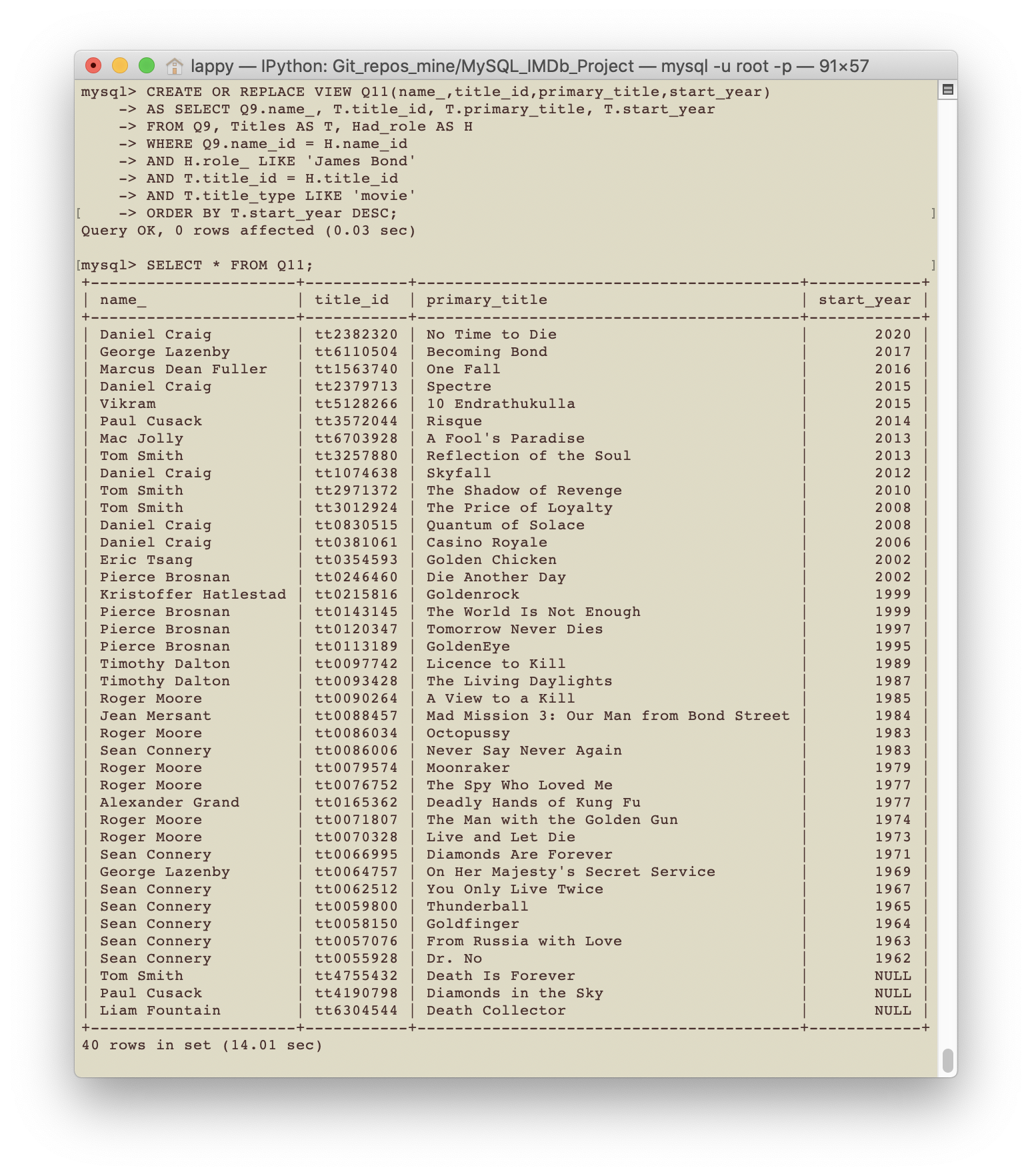
Clearly, a few of these movies contain the character James Bond, but are not the
James Bond movies we have in mind. In particular, the appearance of the movie
Deadly Hands of Kung Fu is quite interesting as it looks to be a 1970’s kung
fu flick. Its IMDb page can be found
here. From this page we quote its synopsis:
“It’s one of the “Bruceploitation” films that were made to cash in on Bruce Lee after his death. The story follows Bruce Lee after he dies and ends up in Hell. Once there, he does the logical thing and opens a gym. After fending off the advances of the King Of Hell’s naked wives, he discovers that the most evil people in Hell are attempting a takeover, so Bruce sets out to stop it. As if it wasn’t weird enough, the evil people are: Zatoichi (the blind swordsman hero of Japanese film), James Bond, The Godfather, The Exorcist, Emmanuelle (the “heroine” of many European softcore porn films), Dracula, and, of course, Clint Eastwood (played by a Chinese guy). Aiding Bruce is The One-Armed Swordsman (hero of kung-fu films), Kain from the U.S. tv series, Kung-Fu (actually played by a Chinese guy this time), and Popeye the Sailor Man! Yes, Popeye the Sailor Man. He eats spinach and helps Bruce fight some mummies.”
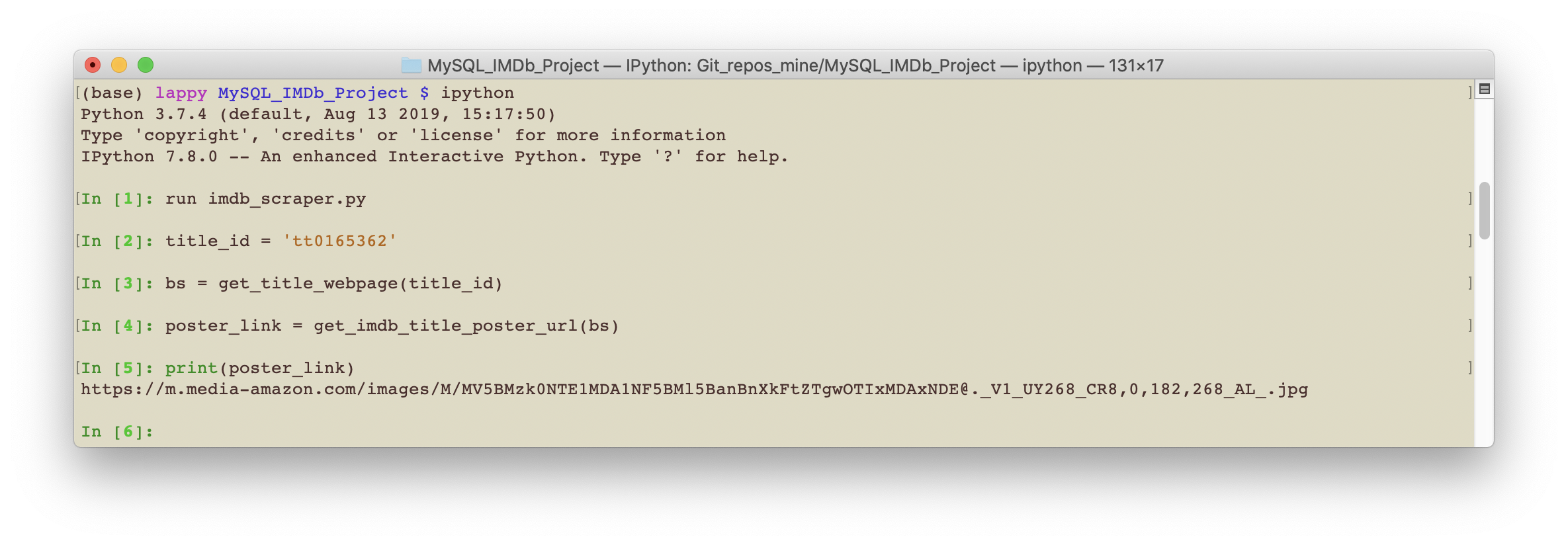
WOW!!! I certainly was not expecting that, I need to see this movie! In the
script imdb_scraper.py we provide a couple of functions that can be used to
extract the url of a movie poster on its IMDb webpage using its title_id.
from bs4 import BeautifulSoup
from urllib.request import urlopen

def get_title_webpage(title_id):
  """
    get_title_webpage(title_id):
    ============================

    Given an IMDb title_id this function will return the title's webpage as
    a BeautifulSoup object.

    INPUT:
    ======

    title_id (string) - An IMDb title id.

    OUTPUT:
    =======

    bs (beaustiful soup object) - The title's webpage as a BeautifulSoup object.

  """

  # Construct url for title
  title_url = 'https://www.imdb.com/title/' + title_id

  # Get the HTML of the title's IMDb page
  html = urlopen(title_url)

  # Create a BeautifulSoup object
  bs = BeautifulSoup(html,"html.parser")

  return bs


def get_imdb_title_poster_url(bs):
  """
    get_imdb_title_poster_url(bs):
    ==============================

    Given a BeautifulSoup object of a title's IMDb webpage this function will
    return the url for its poster.

    INPUT:
    ======

    bs (beaustiful soup object) - The title's webpage as a BeautifulSoup object.

    OUTPUT:
    =======

    poster_link (string) - Link to the poster.

  """

  # Extract poster link
  data = bs.find('div',{'class':'poster'})
  poster_link = data.img['src']

  return poster_link
The functions used to scrape the movie poster url made use of BeautifulSoup and urllib.request. To see how these functions can be used in practice seen the screenshot below.

SQL Queries using python and data visualisation
In the notebook MySQL_IMDb_visualisation.ipynb we query the IMDb database to
explore and visualise the IMDb dataset using pandas and matplotlib.
This notebook is by no means a thorough exploration of the IMDb dataset. Its
purpose is to practice querying a database using python, then to process and
visualise the retrieved data with the pandas package. In particular, we consider
the following questions:
- What are the average ratings for the TV show ‘The X-files’?
- What genres are there?
- How many movies are there in each genre?
- How many movies are made in each genre each year?
- How do the average ages of leading actors and actresses compare in each genre?
- What is a typical runtime for movies in each genre?
This section is also an ongoing piece of work, which will be added to in the future.
To connect to the MySQL IMDb database we use the following code. Of course you will need to use your own password.
import mysql.connector

mydb = mysql.connector.connect(
    host='localhost',
    user='root',
    passwd='put_your_password_here',
    auth_plugin='mysql_native_password',
    database='IMDb')
We then create a cursor.
mycursor = mydb.cursor()
To execute a query we simply use the cursor’s execute and fetchall methods. For example to show all tables in the IMDb database
mycursor.execute("SHOW TABLES;")
tables = mycursor.fetchall()
To print the contents of the tables variable we can simply do the following
print('IMDb Database contains the following tables:')
print('--------------------------------------------')
for table in tables:
    print(table[0])
Since we have ran the SQL script containing many queries, we have many tables in our database.
IMDb Database contains the following tables:
--------------------------------------------
Alias_attributes
Alias_types
Aliases
Directors
Episode_belongs_to
Had_role
Known_for
Leading_people
Name_worked_as
Names_
Principals
q1
q10
q11
q12
q13
q14
q15
q16
q17
q18
q19
q2
q20
q21
q22
q23
q24
q3
q4
q5
q6
q7
q8
q9
Title_genres
Title_ratings
Titles
Writers
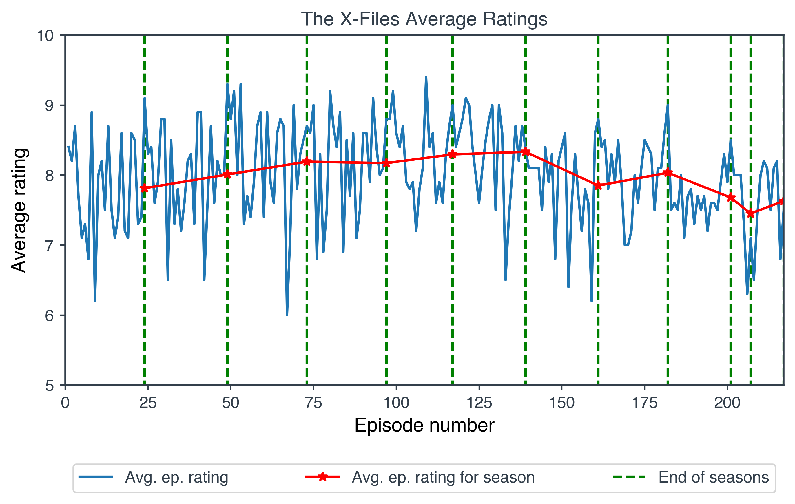
Visualising the ratings of the tv show “The X-Files”
What is the average rating of each episode of The X-Files?
Query1 = """SELECT E.season_number, E.episode_number, T2.primary_title, R.average_rating
FROM Titles AS T1, Titles AS T2, Episode_belongs_to AS E, Title_ratings AS R
WHERE T1.primary_title = 'The X-Files'
AND T1.title_type = 'tvSeries'
AND T1.title_id = E.parent_tv_show_title_id
AND T2.title_type = 'tvEpisode'
AND T2.title_id = E.episode_title_id
AND T2.title_id = R.title_id
ORDER BY E.season_number, E.episode_number;"""

mycursor.execute(Query1)

data = mycursor.fetchall()

df = pd.DataFrame(data,columns=['season_no','episode_no','ep_title','avg_rating'])
How many episodes were there in The X-Files per season? And what was the average of the average episode ratings for each season?
Query2 = """SELECT Q22.season_number, COUNT(*) AS Number_of_episodes, AVG(Q22.average_rating) AS Average_of_ep_average_ratings
FROM Q22
GROUP BY Q22.season_number
ORDER BY Q22.season_number;"""

mycursor.execute(Query2)

data = mycursor.fetchall()

df2 = pd.DataFrame(data,columns=['season_no','no_of_eps','avg_of_avg_ratings'])

df2['total_eps_so_far'] = df2['no_of_eps'].cumsum()
We will plot the results of the above two queries to illustrate the average ratings of The X-files episodes. Please see the notebook for the details of how to produce this figure.
Genres
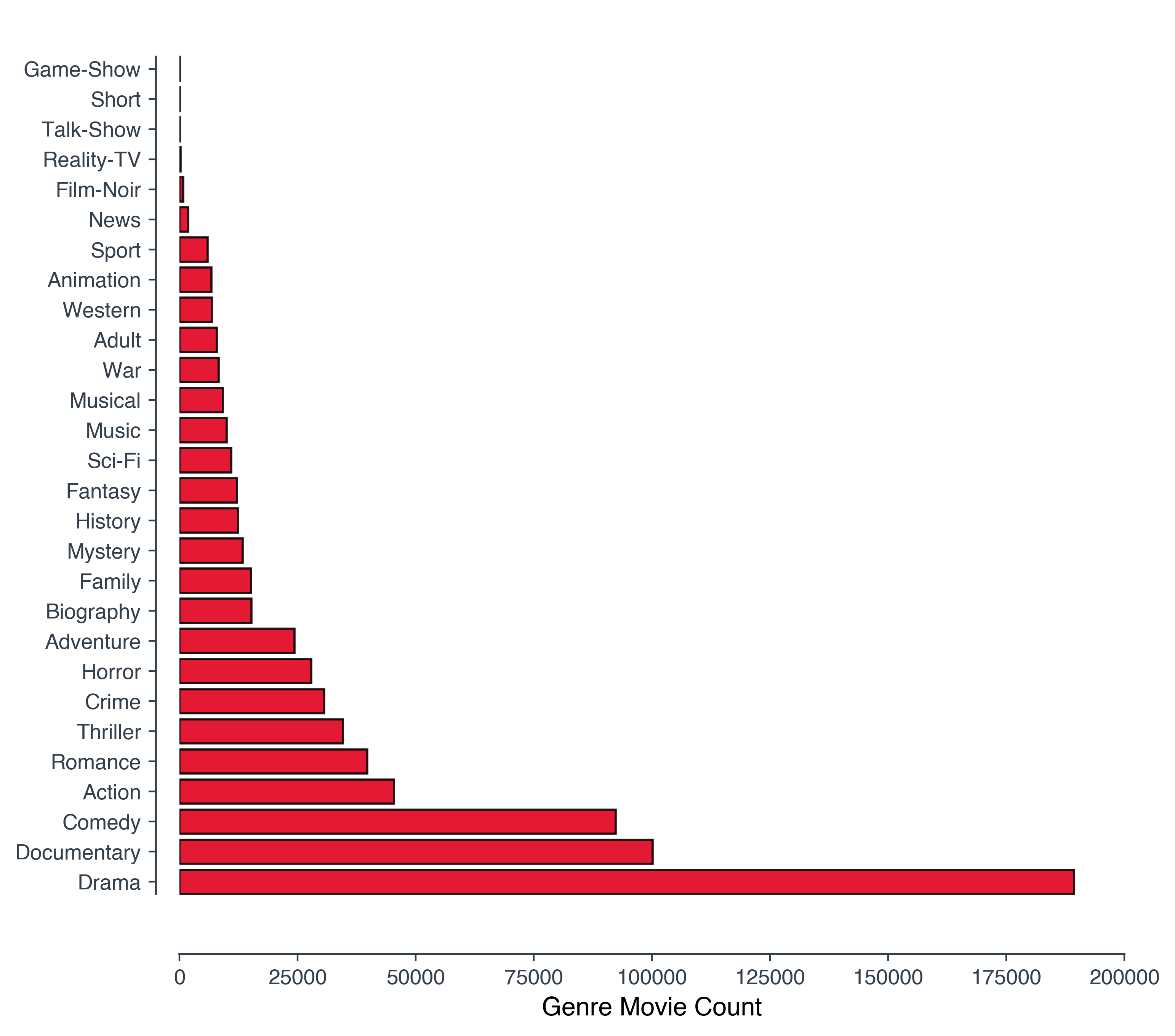
Let’s start with something fairly simple. What genres are there? How many movies are there in each genre?
Query3 ="""SELECT G.genre, COUNT(G.genre) AS Count
FROM Title_genres AS G, Titles AS T
WHERE T.title_id = G.title_id
AND T.title_type = 'movie'
GROUP BY genre
ORDER BY Count DESC;"""

mycursor.execute(Query3)

data = mycursor.fetchall()

df3 = pd.DataFrame(data,columns=['Genre','No. of movies'])
We will visualise this data using a horizontal bar chart.
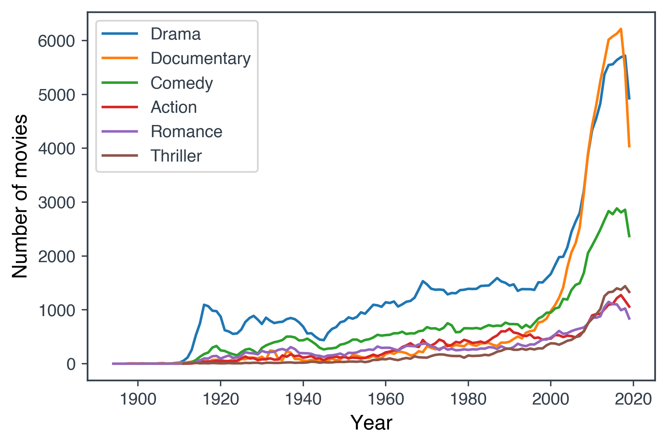
How many movies are made in each genre each year? We only consider up to and including 2019.
Query4 ="""SELECT T.start_year, G.genre, COUNT(DISTINCT T.title_id) AS Number_of_movies
FROM Titles AS T, Title_genres AS G
WHERE T.title_id = G.title_id
AND T.title_type = 'movie'
AND T.start_year <= 2019
GROUP BY T.start_year, G.genre
ORDER BY T.start_year DESC, G.genre ASC;"""

mycursor.execute(Query4)

data = mycursor.fetchall()

df4 = pd.DataFrame(data,columns=['Year','Genre','Number of movies'])
We will visualise this data using a line plot.
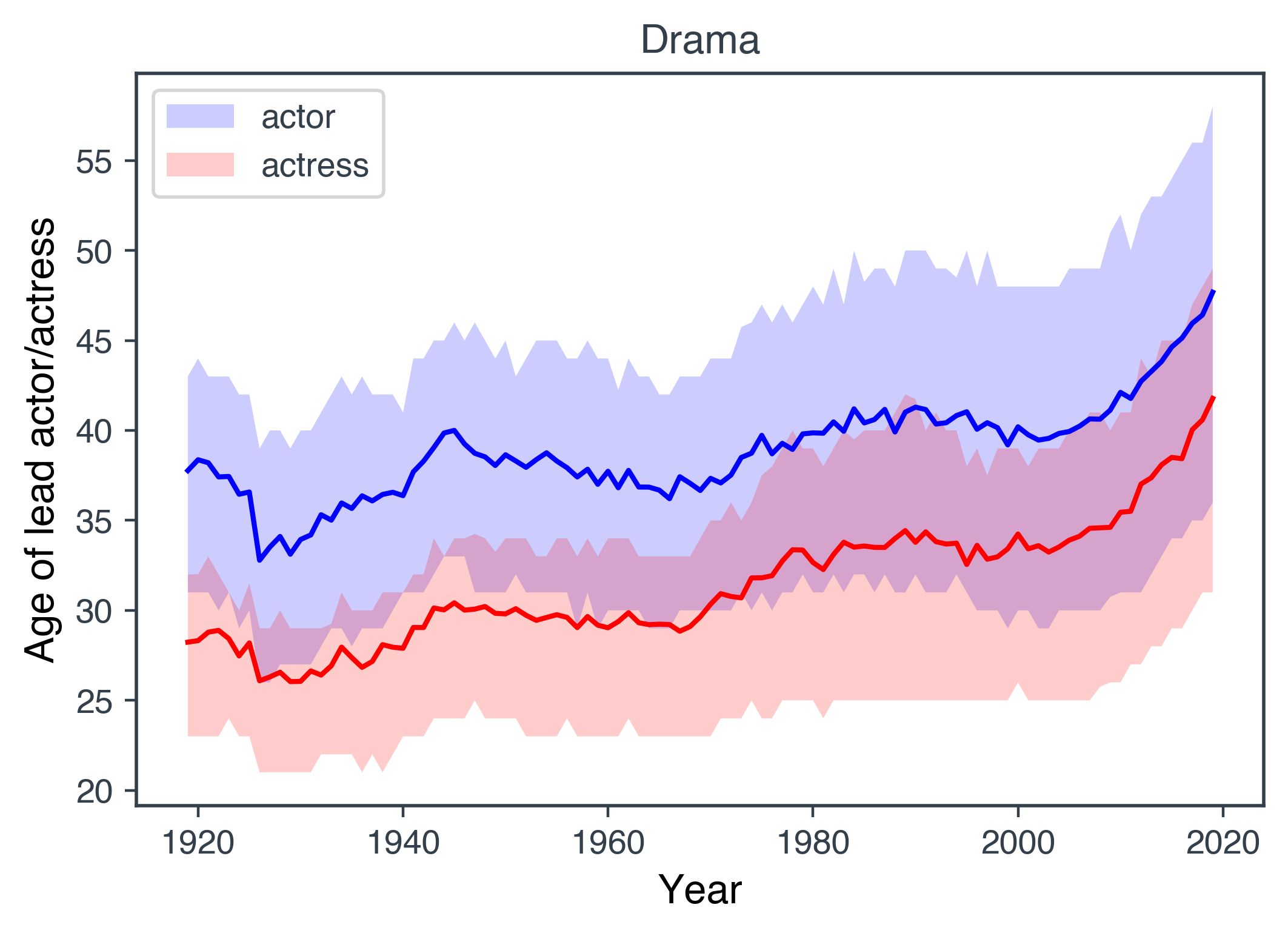
How do the average ages of leading actors and actresses compare in each genre?
We limit ourselves to movies between 1919 and 2019. To determine the age of an actor/actress when the movie was being made the title start year and the birth year of the person must both be non-NULL. If either of these are NULL, then that entry is neglected.
First we create an intermediate table Leading_people with ‘year’,’title_id’,’job_category’, and ‘ordering’ data. We then query this table to combine this with ‘age’ and ‘genre’ information.
Query5 = """CREATE TABLE  Leading_people
AS SELECT T.start_year, T.title_id, P.job_category, MIN(P.ordering) AS ordering
FROM Titles AS T, Principals AS P, Names_ AS N
WHERE T.title_id = P.title_id
AND P.job_category IN ('actor','actress')
AND T.title_type = 'movie'
AND T.start_year IS NOT NULL
AND N.birth_year IS NOT NULL
AND N.name_id = P.name_id
AND T.start_year BETWEEN 1919 AND 2019
GROUP BY T.title_id, P.job_category
ORDER BY T.start_year, T.title_id;"""

mycursor.execute(Query5)

Query6 = """SELECT L.*, T.start_year - N.birth_year AS age, G.genre
FROM Leading_people AS L, Names_ AS N, Titles AS T, Principals AS P, Title_genres AS G
WHERE L.title_id = T.title_id
AND P.title_id = L.title_id
AND P.name_id = N.name_id
AND P.ordering = L.ordering
AND T.title_id = G.title_id ;"""

mycursor.execute(Query6)

data = mycursor.fetchall()

df6 = pd.DataFrame(data,columns=['year','title_id','job_category','ordering','age','genre'])
Let’s group by year, job_category (actor/actress, i.e., gender) and also genre using pandas’ groupby function
df_ages = df6[['year','job_category','genre','age']].groupby(by=['year','job_category','genre'])
We define two functions which will be passed to the aggregrate function. These functions will be used to calculate the first and third quartile.
def Q1(x):
    """The first quartile = 0.25 quantile = 25 th percentile."""
    return x.quantile(q=0.25)

def Q3(x):
    """The third quartile = 0.75 quantile = 75 th percentile."""
    return x.quantile(q=0.75)

df = df_ages.agg({'age': ['mean','median', Q1,Q3]}).reset_index()
````

Rename columns

```python
df.columns = ['year','job_category','genre','mean','median','Q1','Q3']
Let’s visualise this data for just the Drama movies, which is the top genre. The lines are the mean values and the bands are given by the first and third quartiles.
Now let’s visualise for the top 9 genres.
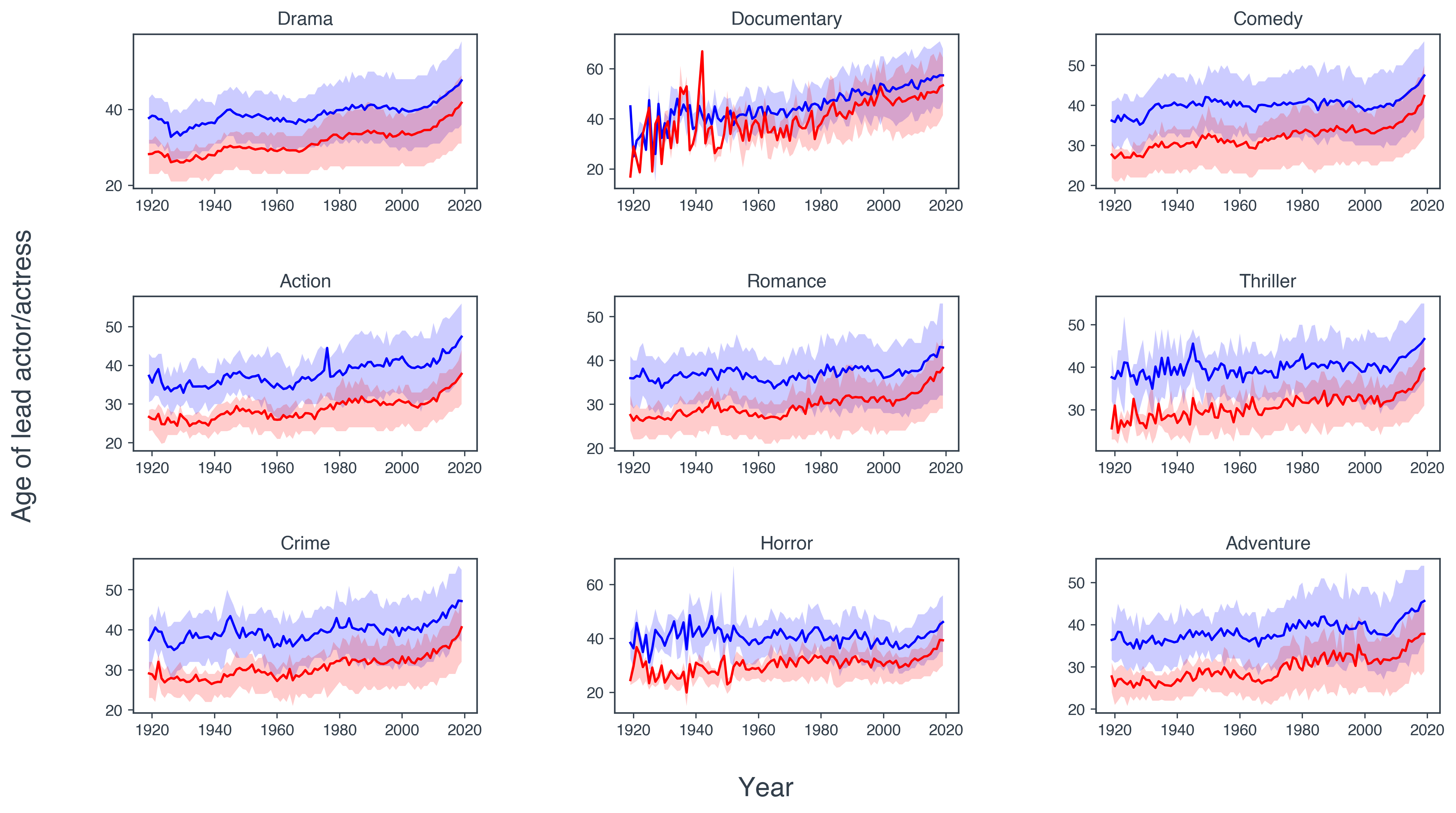
We see a very clear trend in pretty much all genres shown. The leading men are typically older than the leading ladies. Although
this trend is not as clear cut for documentaries.
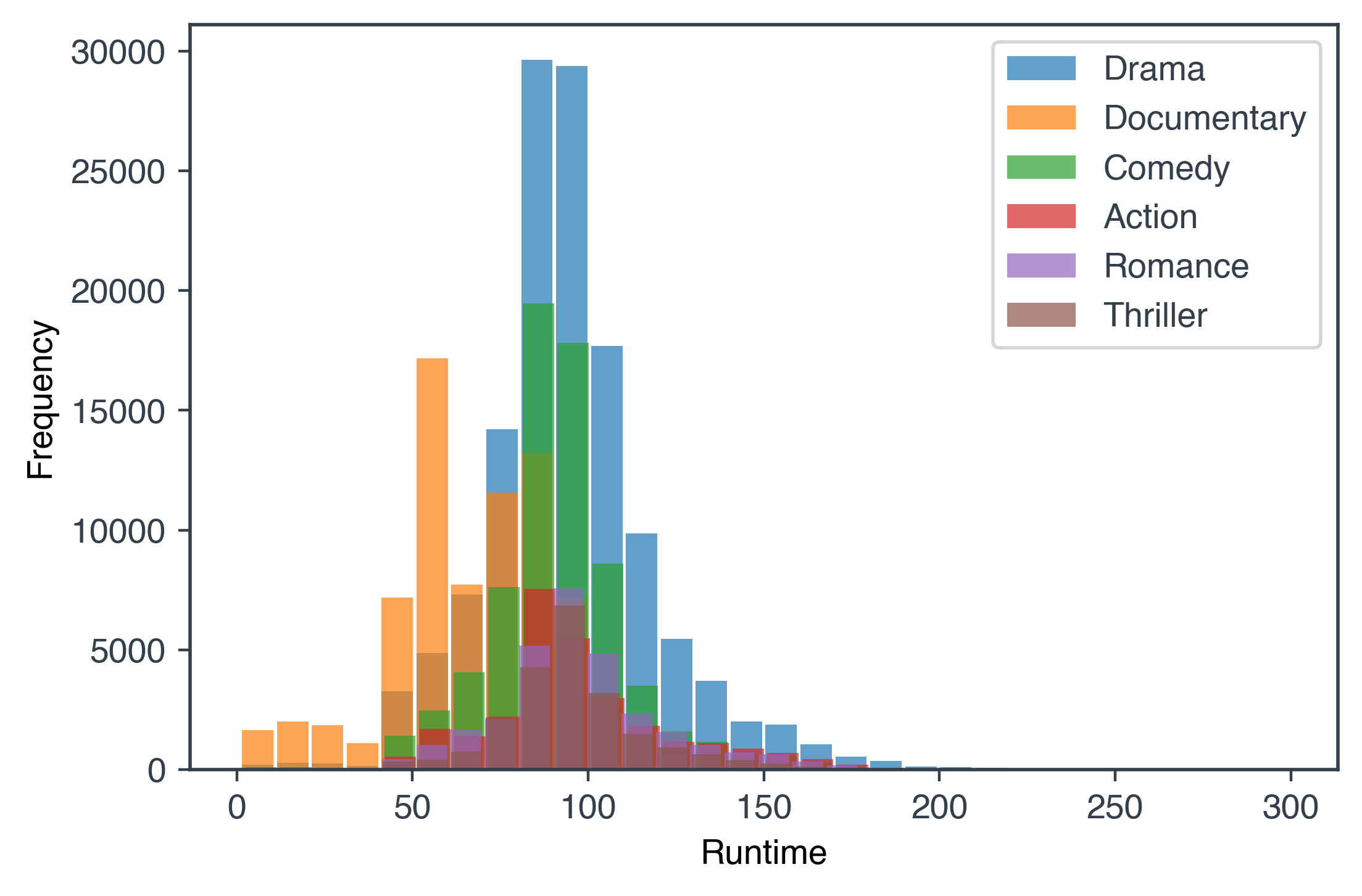
What is a typical runtime for movies in each genre?
Query7 ="""SELECT G.genre, T.runtime_minutes
FROM Titles AS T, Title_genres AS G
WHERE T.runtime_minutes IS NOT NULL
AND T.title_type = 'movie'
AND T.title_id = G.title_id; """

mycursor.execute(Query7)

data = mycursor.fetchall()
Some titles have extremely large and unrealistic values. We choose to ignore these by introducing a cutoff of 300 minutes for the runtime minutes. We visualise this data for 6 genres as a histogram plot.
We finish by closing the connection to the database.
mycursor.close()
mydb.close()
Conclusion
In this post we looked at querying the IMDb database, we created in previous posts, in a few different ways. We then proceeded to visualise the retrieved data. This post was meant to only scratch the surface of what could be done with this data. At a later date we will likely return to this dataset again to try out other ETL tools such as Microsoft’s SQL Server Integrations Services (SSIS) and others. We may also investigate trends further by performing statistical analyses and possibly even use some machine learning algorithms. Well this concludes the series of posts on building and querying a MySQL database for the IMDb dataset.