This is the second in a series of related blog posts/tutorials looking at directional statistics and machine learning. In this second post we will look at the von Mises-Fisher distribution. In particular, we will implement functions to sample from the von Mises-Fisher distribution [1]. Moreover, we will also implement a few functions to visualise spherical data.

In our previous post we looked at the von Mises distribution. In particular, we showed how one could sample from it and how one could visualise circular data. This distribution is available in the scipy statistics package. Numpy also has an implementation as well, which can be found here. However, as we saw in the last post it is quite easy to write your own implementation (see Refs. [2,3]), which may be needed if you are working with a language other than python. However, these libraries don’t implement many other functions related to field of directional statistics and this is something we will be looking at doing in this series. In fact, there isn’t any implementations for the von Mises-Fisher distribution, which is the focus of this tutorial.

Introduction

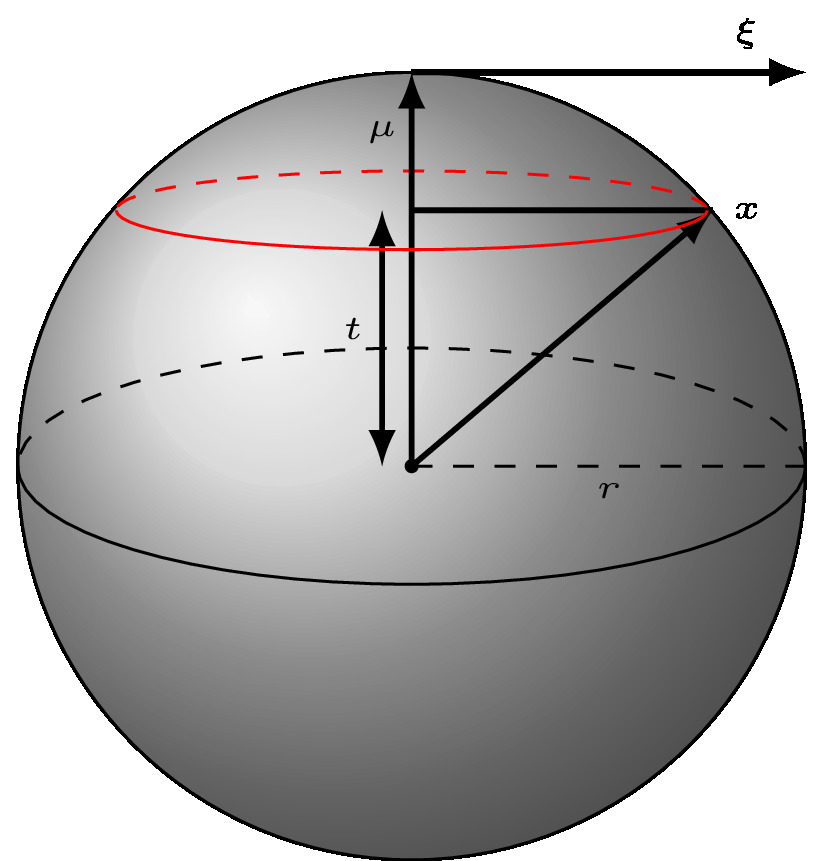
where

is the concentration
is the mean direction and is a unit vector ()
is the random unit vector
is the modified Bessel function of the first kind of order
is the normalisation coefficient which can be shown to be dependent only on and the dimension

A few observations:

the distribution is rotationally symmetric about
If is an orthogonal transformation (), then

A useful property is that under multiplication

where and .

as the clustering about the mean direction increases

A few special cases:

it is the uniform distribution on the -dimensional hypersphere
In the case of the unit sphere the normalisation coefficient simplifies to

,
is the p-dimensional identity matrix,
such that is normal to ,
and we have used pythagorus’ theorem ()
which leads us to

and are independent
is uniform on

Simulation

Ulrich in 1984 [2] gave an algorithm to sample the von Mises-Fisher distribution, which was later improved upon by Wood in 1994 [3]. From the above considerations it is obvious that a von Mises-Fisher sample can be simulated by

generating from the uniform distribution on
generating on the interval from the marginal distribution, which can be shown to be [1]
and then combining them using to produce pseudo-random unit vectors with a von Mises-Fisher distribution

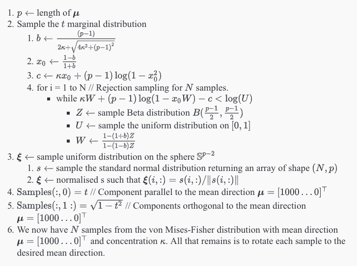
Algorithm

Implementation

Sampling the uniform distribution on a -dimensional hyper-sphere

def rand_uniform_hypersphere(N,p):

    """
        rand_uniform_hypersphere(N,p)
        =============================

        Generate random samples from the uniform distribution on the (p-1)-dimensional
        hypersphere $\mathbb{S}^{p-1} \subset \mathbb{R}^{p}$. We use the method by
        Muller [1], see also Ref. [2] for other methods.

        INPUT:  

            * N (int) - Number of samples
            * p (int) - The dimension of the generated samples on the (p-1)-dimensional hypersphere.
                - p = 2 for the unit circle $\mathbb{S}^{1}$
                - p = 3 for the unit sphere $\mathbb{S}^{2}$
            Note that the (p-1)-dimensional hypersphere $\mathbb{S}^{p-1} \subset \mathbb{R}^{p}$ and the
            samples are unit vectors in $\mathbb{R}^{p}$ that lie on the sphere $\mathbb{S}^{p-1}$.

    References:

    [1] Muller, M. E. "A Note on a Method for Generating Points Uniformly on N-Dimensional Spheres."
    Comm. Assoc. Comput. Mach. 2, 19-20, Apr. 1959.

    [2] https://mathworld.wolfram.com/SpherePointPicking.html

    """

    if (p<=0) or (type(p) is not int):
        raise Exception("p must be a positive integer.")

    # Check N>0 and is an int
    if (N<=0) or (type(N) is not int):
        raise Exception("N must be a non-zero positive integer.")

    v = np.random.normal(0,1,(N,p))

    v = np.divide(v,np.linalg.norm(v,axis=1,keepdims=True))

    return v

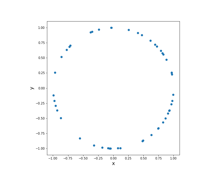
Consider the special case of the unit circle ( )

Generate 50 samples of the uniform distribution on the unit circle.

data = rand_uniform_hypersphere(N=50,p=2)

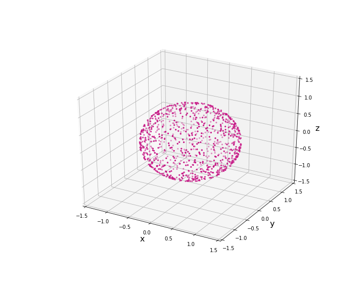
Consider the case of unit sphere ( )

Generate 1000 samples of the uniform distribution on the unit sphere.

data3D = rand_uniform_hypersphere(N=1000,p=3)

Sampling the marginal distribution of using rejections sampling

As mentioned above we use rejection sampling to sample the marginal distribution.

def rand_t_marginal(kappa,p,N=1):
    """
        rand_t_marginal(kappa,p,N=1)
        ============================

        Samples the marginal distribution of t using rejection sampling of Wood [3].

        INPUT:

            * kappa (float) - concentration        
            * p (int) - The dimension of the generated samples on the (p-1)-dimensional hypersphere.
                - p = 2 for the unit circle $\mathbb{S}^{1}$
                - p = 3 for the unit sphere $\mathbb{S}^{2}$
            Note that the (p-1)-dimensional hypersphere $\mathbb{S}^{p-1} \subset \mathbb{R}^{p}$ and the
            samples are unit vectors in $\mathbb{R}^{p}$ that lie on the sphere $\mathbb{S}^{p-1}$.
            * N (int) - number of samples

        OUTPUT:

            * samples (array of floats of shape (N,1)) - samples of the marginal distribution of t
    """

    # Check kappa >= 0 is numeric
    if (kappa < 0) or ((type(kappa) is not float) and (type(kappa) is not int)):
        raise Exception("kappa must be a non-negative number.")

    if (p<=0) or (type(p) is not int):
        raise Exception("p must be a positive integer.")

    # Check N>0 and is an int
    if (N<=0) or (type(N) is not int):
        raise Exception("N must be a non-zero positive integer.")


    # Start of algorithm
    b = (p - 1.0) / (2.0 * kappa + np.sqrt(4.0 * kappa**2 + (p - 1.0)**2 ))    
    x0 = (1.0 - b) / (1.0 + b)
    c = kappa * x0 + (p - 1.0) * np.log(1.0 - x0**2)

    samples = np.zeros((N,1))

    # Loop over number of samples
    for i in range(N):

        # Continue unil you have an acceptable sample
        while True:

            # Sample Beta distribution
            Z = np.random.beta( (p - 1.0)/2.0, (p - 1.0)/2.0 )

            # Sample Uniform distribution
            U = np.random.uniform(low=0.0,high=1.0)

            # W is essentially t
            W = (1.0 - (1.0 + b) * Z) / (1.0 - (1.0 - b) * Z)

            # Check whether to accept or reject
            if kappa * W + (p - 1.0)*np.log(1.0 - x0*W) - c >= np.log(U):

                # Accept sample
                samples[i] = W
                break

    return samples

Finally, we can put it all together to sample the von Mises-Fisher distribution.

def rand_von_mises_fisher(mu,kappa,N=1):
    """
        rand_von_mises_fisher(mu,kappa,N=1)
        ===================================

        Samples the von Mises-Fisher distribution with mean direction mu and concentration kappa.

        INPUT:

            * mu (array of floats of shape (p,1)) - mean direction. This should be a unit vector.
            * kappa (float) - concentration.
            * N (int) - Number of samples.

        OUTPUT:

            * samples (array of floats of shape (N,p)) - samples of the von Mises-Fisher distribution
            with mean direction mu and concentration kappa.
    """


    # Check that mu is a unit vector
    eps = 10**(-8) # Precision
    norm_mu = np.linalg.norm(mu)
    if abs(norm_mu - 1.0) > eps:
        raise Exception("mu must be a unit vector.")

    # Check kappa >= 0 is numeric
    if (kappa < 0) or ((type(kappa) is not float) and (type(kappa) is not int)):
        raise Exception("kappa must be a non-negative number.")

    # Check N>0 and is an int
    if (N<=0) or (type(N) is not int):
        raise Exception("N must be a non-zero positive integer.")

    # Dimension p
    p = len(mu)

    # Make sure that mu has a shape of px1
    mu = np.reshape(mu,(p,1))

    # Array to store samples
    samples = np.zeros((N,p))

    #  Component in the direction of mu (Nx1)
    t = rand_t_marginal(kappa,p,N)

    # Component orthogonal to mu (Nx(p-1))
    xi = rand_uniform_hypersphere(N,p-1)

    # von-Mises-Fisher samples Nxp

    # Component in the direction of mu (Nx1).
    # Note that here we are choosing an
    # intermediate mu = [1, 0, 0, 0, ..., 0] later
    # we rotate to the desired mu below
    samples[:,[0]] = t

    # Component orthogonal to mu (Nx(p-1))
    samples[:,1:] = np.matlib.repmat(np.sqrt(1 - t**2), 1, p-1) * xi

    # Rotation of samples to desired mu
    O = null_space(mu.T)
    R = np.concatenate((mu,O),axis=1)
    samples = np.dot(R,samples.T).T

    return samples

Consider the case of unit sphere ( )

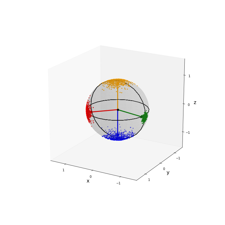
We now create four sets of samples with different mean direction and concentration. Each set will have 500 samples. Note that we have normalised our mean direction vectors to be unit vectors. This normalisation is required by rand_von_mises_fisher().

# All sets have the same number of data points
Nsim = 500

# Set 1
mu1 = [1,1,0]
mu1 = mu1/np.linalg.norm(mu1)
kappa1 = 50
data1 = rand_von_mises_fisher(mu1,kappa=kappa1,N=Nsim)

# Set 2
mu2 = [0,0,1]
mu2 = mu2/np.linalg.norm(mu2)
kappa2 = 20
data2 = rand_von_mises_fisher(mu2,kappa=kappa2,N=Nsim)

# Set 3
mu3 = [0,0,-1]
mu3 = mu3/np.linalg.norm(mu3)
kappa3 = 20
data3 = rand_von_mises_fisher(mu3,kappa=kappa3,N=Nsim)

# Set 4
mu4 = [-10,0,-1]
mu4 = mu4/np.linalg.norm(mu4)
kappa4 = 200
data4 = rand_von_mises_fisher(mu4,kappa=kappa4,N=Nsim)

To visual this data we have written two functions to accomplish this. The main function is plot_3d_scatter(), which is used to plot the 3D samples and a transparent sphere. The second is plot_arrow() (see associated repository) used to plot arrows in the mean direction of the samples.

def plot_3d_scatter(data,ax=None,colour='red',sz=30,el=20,az=50,sph=True,sph_colour="gray",sph_alpha=0.03,
                    eq_line=True,pol_line=True,grd=False):
    """
        plot_3d_scatter()
        =================

        Plots 3D samples on the surface of a sphere.

        INPUT:

            * data (array of floats of shape (N,3)) - samples of a spherical distribution such as von Mises-Fisher.
            * ax (axes) - axes on which the plot is constructed.
            * colour (string) - colour of the scatter plot.
            * sz (float) - size of points.
            * el (float) - elevation angle of the plot.
            * az (float) - azimuthal angle of the plot.
            * sph (boolean) - whether or not to inclde a sphere.
            * sph_colour (string) - colour of the sphere if included.
            * sph_alpha (float) - the opacity/alpha value of the sphere.
            * eq_line (boolean) - whether or not to include an equatorial line.
            * pol_line (boolean) - whether or not to include a polar line.
            * grd (boolean) - whether or not to include a grid.

        OUTPUT:

            * ax (axes) - axes on which the plot is contructed.
            * Plot of 3D samples on the surface of a sphere.

    """


    # The polar axis
    if ax is None:
        ax = plt.axes(projection='3d')

    # Check that data is 3D (data should be Nx3)
    d = np.shape(data)[1]
    if d != 3:
        raise Exception("data should be of shape Nx3, i.e., each data point should be 3D.")

    ax.scatter(data[:,0],data[:,1],data[:,2],s=5,c=colour)
    ax.view_init(el, az)
    ax.set_xlim(-1.5,1.5)
    ax.set_ylim(-1.5,1.5)
    ax.set_zlim(-1.5,1.5)

    # Add a shaded unit sphere
    if sph:
        u, v = np.mgrid[0:2*np.pi:30j, 0:np.pi:30j]
        x = np.cos(u)*np.sin(v)
        y = np.sin(u)*np.sin(v)
        z = np.cos(v)
        ax.plot_surface(x, y, z, color=sph_colour,alpha=sph_alpha)

    # Add an equitorial line
    if eq_line:
        # t = theta, p = phi
        eqt = np.linspace(0,2*np.pi,50,endpoint=False)
        eqp = np.linspace(0,2*np.pi,50,endpoint=False)
        eqx = 2*np.sin(eqt)*np.cos(eqp)
        eqy = 2*np.sin(eqt)*np.sin(eqp) - 1
        eqz = np.zeros(50)

        # Equator line
        ax.plot(eqx,eqy,eqz,color="k",lw=1)

    # Add a polar line
    if pol_line:
        # t = theta, p = phi
        eqt = np.linspace(0,2*np.pi,50,endpoint=False)
        eqp = np.linspace(0,2*np.pi,50,endpoint=False)
        eqx = 2*np.sin(eqt)*np.cos(eqp)
        eqy = 2*np.sin(eqt)*np.sin(eqp) - 1
        eqz = np.zeros(50)

        # Polar line
        ax.plot(eqx,eqz,eqy,color="k",lw=1)

    # Draw a centre point
    ax.scatter([0], [0], [0], color="k", s=sz)    

    # Turn off grid
    ax.grid(grd)

    # Ticks
    ax.set_xticks([-1,0,1])
    ax.set_yticks([-1,0,1])
    ax.set_zticks([-1,0,1])

    return ax

Putting these together we visualise the four sets of samples. Note that the samples on the far side of the sphere are of a lighter shade to exhibit the fact they are on the other side of the sphere.

fig = plt.figure(figsize=(10,10))
ax = plt.axes(projection='3d')

# Set 1
plot_3d_scatter(data1,ax)
plot_arrow(mu1,ax,colour="red")

# Set 2
plot_3d_scatter(data2,ax,colour='orange')
plot_arrow(mu2,ax,colour="orange")

# Set 3
plot_3d_scatter(data3,ax,colour='blue')
plot_arrow(mu3,ax,colour="blue")

# Set 4
plot_3d_scatter(data4,ax,colour='green')
plot_arrow(mu4,ax,colour="green")

# Labels
ax.set_xlabel('x',fontsize=fs)
ax.set_ylabel('y',fontsize=fs)
ax.set_zlabel('z',fontsize=fs)

# Viewing angle
ax.view_init(20,120)

If you want to make the 3D image interactive in the jupyter notebook, so you can rotate to a better angle. This is easily done by including the command

%matplotlib notebook

before plotting the image. If you want to revert back, simply use

%matplotlib inline

Concluding remarks

The analysis of circular and more generally directional data is extremely important to many fields of study, but it is rarely given the same amount of attention as statistics in Euclidean spaces. This is the second in a series of tutorials looking at topics in directional statistics and machine learning. Today we looked at one of the most important hyper-spherical distributions which has many applications ranging from astrophysics to paleomagnetism. We presented how one might sample the von Mises-Fisher distribution. This is important because there are no implementations available in the usual python libraries. We also showed how one can visualise spherical data. In later tutorials we will consider other important directional distributions and machine learning algorithms which make use of them.

Please note not all code is given in the blog article. For all code including all supporting functions please see the associated repository.

References

Mardia, K.V. and Jupp, P.E., Directional Statistics. John Wiley & Sons, London (2000).
Ulrich, G., Computer Generation of Distributions on the m-sphere, Appl. Statist. 33, No. 2. pp. 158-163, (1984).
Wood, A. T. A., Simulation of the von Mises Fisher distribution, Communications in Statistics - Simulation and Computation, 23 , 157-164 (1994).
https://mathworld.wolfram.com/SpherePointPicking.html
Muller, M. E.“A Note on a Method for Generating Points Uniformly on N-Dimensional Spheres.” Comm. Assoc. Comput. Mach. 2, 19-20, Apr. (1959).
Hornik, Kurt and Grün, Bettina, movMF: An R Package for Fitting Mixtures of von Mises-Fisher Distributions, Journal of Statistical Software, 58 (10), pp. 1-31 (2014).
Drawing a fancy vector see https://stackoverflow.com/questions/11140163/plotting-a-3d-cube-a-sphere-and-a-vector-in-matplotlib